
In this article, we will help you understand cycle time in ESP Analytics.
|
Skip Ahead to: |
Overview
Cycle time is defined here as the difference between the exit time and the corresponding entry time of a card, that is the time spent in the selected region of the value stream during that visit. In a normal situation, as cards move forward from left to right, a card will travel through the selected region of the value stream only once. However, if we allow cards to move back, or move between different value streams (swim lanes) it is possible for a card to visit multiple times. In such situations, the scatter plot will show multiple instances of the card, once for each visit.
Applying Filters
You can apply filters based on card attributes and the value stream stages to refine your data for the analytics. Moreover, the time range for the analytics can also be adjusted using the Temporal Range Filter. Read more about them here.
Cycle Time Scatter Plot
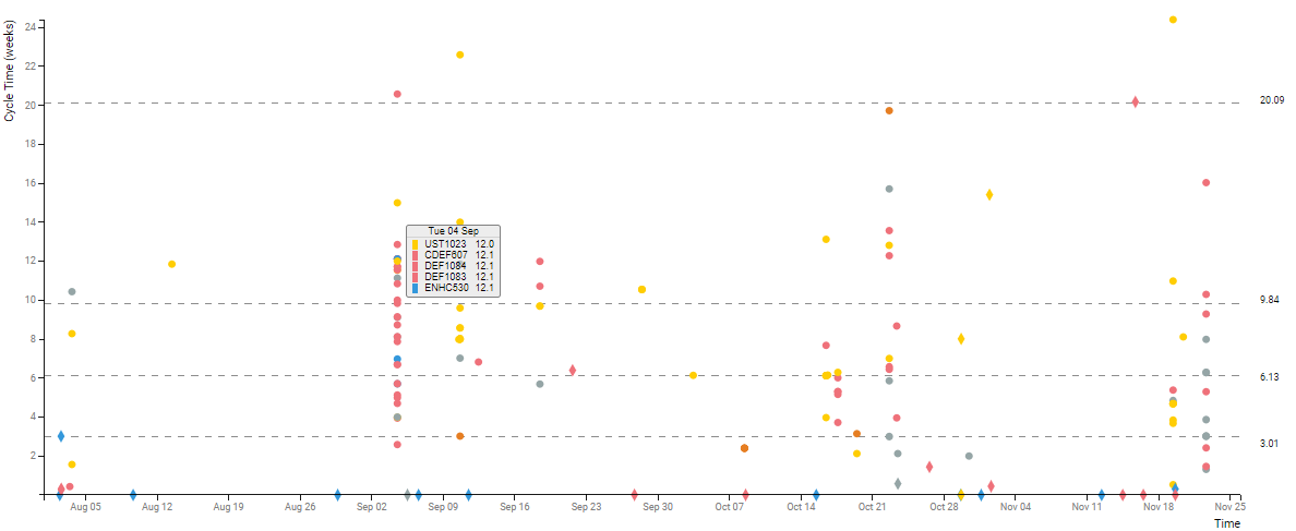
The x-axis represents time, the y-axis represents cycle time (in units selected in Time Unit filter criteria). Each dot represents a card whose x position is determined by its exit time, and whose y position is determined by the cycle time. The dots are colored based on the value of Color by attribute of the card. Different shapes indicate the type of exit:
- Circle: move forward or is archived
- Triangle: move back
- Square: move to another value stream
- Diamond: cards that were deleted or discarded
You can further analyze the Scatterplot data based on the Quartile or the Percentile value and also view the Rolling average line for a user-driven number of days. To view such data, click the ![]() icon from the widget menu, and then select any of the following options:
icon from the widget menu, and then select any of the following options:
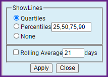
Quartile
On the right of the scatter plot, we have a box-and-whisker plot as defined by John W. Tukey. Box-plot provides a non-parametric characterization of data without making any assumptions of the underlying distribution. The bottom and top of the box are the first and third quartiles, and the line inside the box is the second quartile (the median). The lower whiskers are drawn to the lowest datum still within the 1.5 IRQ ( interquartile range: q3 – q1) of the lower quartile, and the upper whisker is the highest datum still within the 1.5 IRQ of the upper quartile.
Box-and-whisker plot is often used to identify outliers in place of 3 sigmas when the underlying distribution is unknown. For comparison, for normal distribution, the 6 sigma range represents 99.73% of the total area, whereas the box-and-whisker range represents 99.3% of the area. The actual area being covered, however, depends on the nature of the distribution.
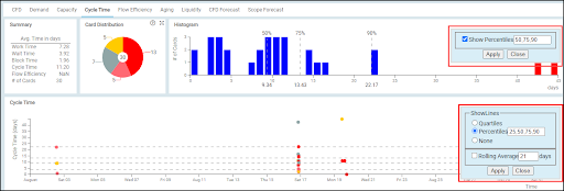
Percentile
you enter the percentile values as per your requirement with the comma-separated format, the horizontal dotted lines demarcate the area of observation. Each area between the dotted lines represents the percentile value below which a percentage of average cycle time data falls.
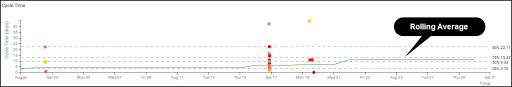
Rolling Average
You can plot a line based on the rolling average of the cycle time for the n number of days. The rolling average is the moving average of the cards that exit the selected region of the value stream during the selected time interval. The line is formed by joining the series of data points of the average cycle time for a given time interval. It not only helps you understand the trend of the cards getting done but also visualize the emerging pattern and detect any intermittent peak.
Calculation Logic for the Scatter Plot
Cards that exit the selected region of the value stream during the time interval selected in the Temporal Range Filter, pass the filtering criteria and have entry time defined form the basis for cycle time calculation. These cards are plotted on the chart based on their exit time (x-axis) and cycle time (y-axis).
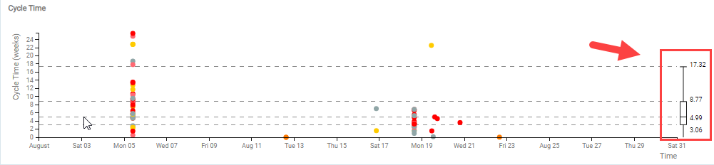
Card Distribution Pie Chart
A pie chart showing the breakdown of cards used in cycle time calculation colored by the Color attribute of the card.
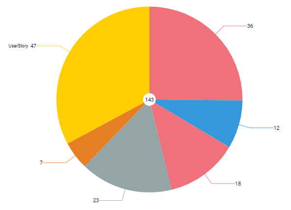
Calculation Logic for the Card Distribution
Cards that exit the selected region of the value stream during the time interval selected in the Temporal Range Filter, pass the filtering criteria and have entry time defined form the basis for cycle time calculation. For the pie chart, these cards are grouped by Color by attribute to form segments of the pie. The total number is shown at the center of the pie.
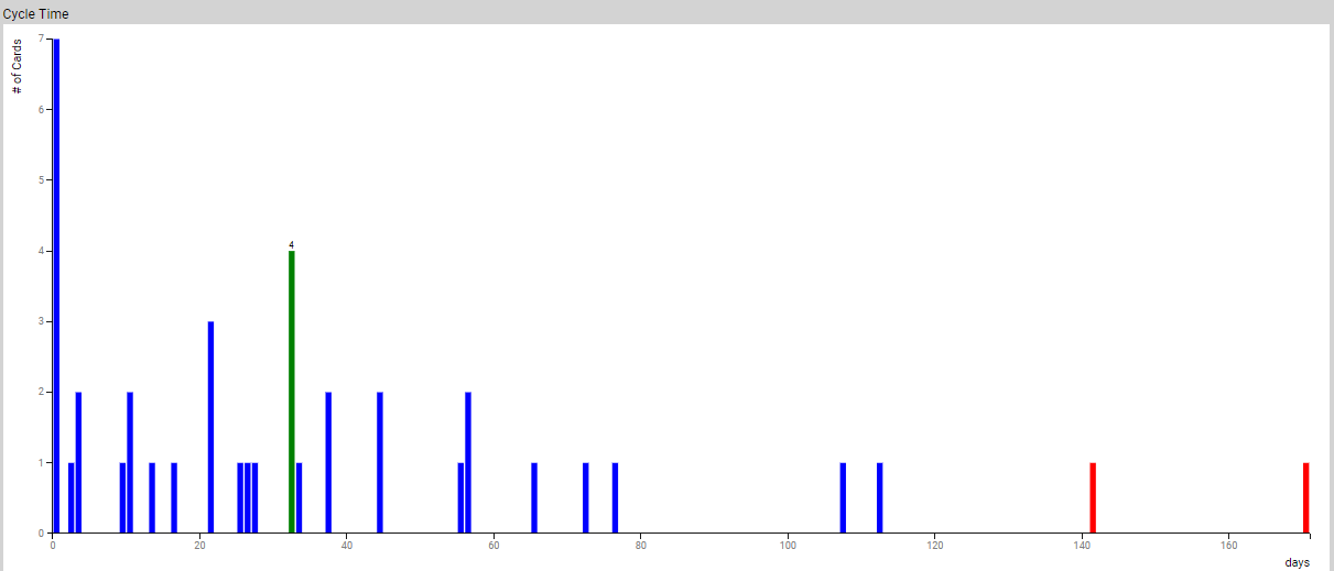
Cycle Time Histogram
It is the histogram of cycle time where the x-axis is the cycle time, and the y-axis represents the number of cards that have cycle time that falls within the time bucket representing the width of the bar. The outliers are colored in red.
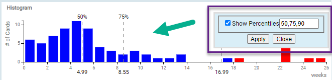
You can further analyze the Histogram data based on the Percentile value. To view such data, click the ![]() icon from the widget menu, and then select the Show Percentile checkbox, and enter your percentile value in the comma-separated format. The vertical dotted lines are displayed that demarcate the area of observation. Each area between the dotted lines represents the percentile value below which a percentage of average cycle time data falls.
icon from the widget menu, and then select the Show Percentile checkbox, and enter your percentile value in the comma-separated format. The vertical dotted lines are displayed that demarcate the area of observation. Each area between the dotted lines represents the percentile value below which a percentage of average cycle time data falls.
Calculation Logic for Cycle Time
Cards that exit the selected region of the value stream during the time interval selected in the Temporal Range Filter, pass the filtering criteria and have entry time defined form the basis for cycle time calculation. These cards are grouped into Time unit-wide buckets based on their cycle time to form the histogram. Cards that fall outside the box-and-wiser plot are considered to be outliers and are colored in red.